The law of averages in simple terms. Average values. Weak law of large numbers

The words about large numbers refer to the number of tests - a large number of values ​​​​of a random variable or the cumulative action of a large number of random variables are considered. The essence of this law is as follows: although it is impossible to predict what value a single random variable will take in a single experiment, however, the total result of the action of a large number of independent random variables loses its random character and can be predicted almost reliably (i.e. with high probability). For example, it is impossible to predict which side a coin will fall on. However, if you toss 2 tons of coins, then with great certainty it can be argued that the weight of the coins that fell with the coat of arms up is 1 ton.

First of all, the so-called Chebyshev inequality refers to the law of large numbers, which estimates in a separate test the probability of a random variable accepting a value that deviates from the average value by no more than a given value.

Chebyshev's inequality. Let X is an arbitrary random variable, a=M(X) , a D(X) is its dispersion. Then

Example. The nominal (i.e. required) value of the diameter of the sleeve machined on the machine is 5mm, and the variance is not more than 0.01 (this is the accuracy tolerance of the machine). Estimate the probability that in the manufacture of one bushing, the deviation of its diameter from the nominal will be less than 0.5mm .

Solution. Let r.v. X- the diameter of the manufactured bushing. By condition, its mathematical expectation is equal to the nominal diameter (if there is no systematic failure in setting up the machine): a=M(X)=5 , and the variance D(X)≤0.01. Applying the Chebyshev inequality for ε = 0.5, we get:

Thus, the probability of such a deviation is quite high, and therefore we can conclude that in the case of a single production of a part, the deviation of the diameter from the nominal one will almost certainly not exceed 0.5mm .

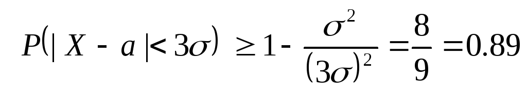
Basically, the standard deviation σ characterizes average deviation of a random variable from its center (i.e. from its mathematical expectation). Because it average deviation, then large deviations (emphasis on o) are possible during testing. How large deviations are practically possible? When studying normally distributed random variables, we derived the “three sigma” rule: a normally distributed random variable X in a single test practically does not deviate from its average further than 3σ, where σ= σ(X) is the standard deviation of r.v. X. We deduced such a rule from the fact that we obtained the inequality

.

Let us now estimate the probability for arbitrary random variable X accept a value that differs from the mean by no more than three times the standard deviation. Applying the Chebyshev inequality for ε = 3σ and given that D(X)=σ 2 , we get:

.

In this way, in general we can estimate the probability of a random variable deviating from its mean by no more than three standard deviations by the number 0.89 , while for a normal distribution it can be guaranteed with probability 0.997 .

Chebyshev's inequality can be generalized to a system of independent identically distributed random variables.

Generalized Chebyshev's inequality. If independent random variables X 1 , X 2 , … , X n M(X i )= a and dispersions D(X i )= D, then

At n=1 this inequality goes over into the Chebyshev inequality formulated above.

The Chebyshev inequality, having independent significance for solving the corresponding problems, is used to prove the so-called Chebyshev theorem. We first describe the essence of this theorem and then give its formal formulation.

Let X 1 , X 2 , … , X n– a large number of independent random variables with mathematical expectations M(X 1 )=a 1 , … , M(X n )=a n. Although each of them, as a result of the experiment, can take a value far from its average (i.e., mathematical expectation), however, a random variable
, equal to their arithmetic mean, with a high probability will take a value close to a fixed number
(this is the average of all mathematical expectations). This means the following. Let, as a result of the test, independent random variables X 1 , X 2 , … , X n(there are a lot of them!) have taken the values ​​accordingly X 1 , X 2 , … , X n respectively. Then if these values ​​themselves may turn out to be far from the average values ​​of the corresponding random variables, their average value
is likely to be close to
. Thus, the arithmetic mean of a large number of random variables already loses its random character and can be predicted with great accuracy. This can be explained by the fact that random deviations of the values X i from a i can be of different signs, and therefore in total these deviations are compensated with a high probability.

Terema Chebyshev (law of large numbers in the form of Chebyshev). Let X 1 , X 2 , … , X n … is a sequence of pairwise independent random variables whose variances are limited to the same number. Then, no matter how small the number ε we take, the probability of inequality

will be arbitrarily close to unity if the number n random variables to take large enough. Formally, this means that under the conditions of the theorem

This type of convergence is called convergence in probability and is denoted by:

Thus, the Chebyshev theorem says that if there are a sufficiently large number of independent random variables, then their arithmetic mean in a single test will almost certainly take a value close to the average of their mathematical expectations.

Most often, the Chebyshev theorem is applied in a situation where random variables X 1 , X 2 , … , X n … have the same distribution (i.e. the same distribution law or the same probability density). In fact, this is just a large number of instances of the same random variable.

Consequence(of the generalized Chebyshev inequality). If independent random variables X 1 , X 2 , … , X n … have the same distribution with mathematical expectations M(X i )= a and dispersions D(X i )= D, then

, i.e.
.

The proof follows from the generalized Chebyshev inequality by passing to the limit as n→∞ .

We note once again that the equalities written above do not guarantee that the value of the quantity
tends to a at n→∞. This value is still a random variable, and its individual values ​​can be quite far from a. But the probability of such (far from a) values ​​with increasing n tends to 0.

Comment. The conclusion of the corollary is obviously also valid in the more general case when the independent random variables X 1 , X 2 , … , X n … have a different distribution, but the same mathematical expectations (equal a) and the variances limited in the aggregate. This makes it possible to predict the accuracy of measuring a certain quantity, even if these measurements are made by different instruments.

Let us consider in more detail the application of this corollary to the measurement of quantities. Let's use some device n measurements of the same quantity, the true value of which is a and we don't know. The results of such measurements X 1 , X 2 , … , X n may differ significantly from each other (and from the true value a) due to various random factors (pressure drops, temperatures, random vibration, etc.). Consider the r.v. X- instrument reading for a single measurement of a quantity, as well as a set of r.v. X 1 , X 2 , … , X n- instrument reading at the first, second, ..., last measurement. Thus, each of the quantities X 1 , X 2 , … , X n there is just one of the instances of the r.v. X, and therefore they all have the same distribution as the r.v. X. Since the measurement results are independent of each other, the r.v. X 1 , X 2 , … , X n can be considered independent. If the device does not give a systematic error (for example, zero is not “knocked down” on the scale, the spring is not stretched, etc.), then we can assume that the mathematical expectation M(X) = a, and therefore M(X 1 ) = ... = M(X n ) = a. Thus, the conditions of the above corollary are satisfied, and therefore, as an approximate value of the quantity a we can take the "implementation" of a random variable
in our experiment (consisting of a series of n measurements), i.e.

.

With a large number of measurements, it is practically reliable good accuracy calculations using this formula. This is the rationale for the practical principle that, with a large number of measurements, their arithmetic mean practically does not differ much from the true value of the measured quantity.

The “sampling” method, which is widely used in mathematical statistics, is based on the law of large numbers, which allows obtaining its objective characteristics with acceptable accuracy from a relatively small sample of values ​​of a random variable. But this will be discussed in the next section.

Example. On a measuring device that does not make systematic distortions, a certain quantity is measured a once (received value X 1 ), and then 99 more times (the values X 2 , … , X 100 ). For the true value of measurement a first take the result of the first measurement
, and then the arithmetic mean of all measurements
. The measurement accuracy of the device is such that the standard deviation of the measurement σ is not more than 1 (because the dispersion D=σ 2 also does not exceed 1). For each of the measurement methods, estimate the probability that the measurement error does not exceed 2.

Solution. Let r.v. X- instrument reading for a single measurement. Then by condition M(X)=a. To answer the questions posed, we apply the generalized Chebyshev inequality

for ε =2 first for n=1 and then for n=100 . In the first case, we get
, and in the second. Thus, the second case practically guarantees the given measurement accuracy, while the first one leaves serious doubts in this sense.

Let us apply the above statements to the random variables that arise in the Bernoulli scheme. Let us recall the essence of this scheme. Let it be produced n independent tests, in each of which some event BUT can appear with the same probability R, a q=1–r(by meaning, this is the probability of the opposite event - not the occurrence of an event BUT) . Let's spend some number n such tests. Consider random variables: X 1 – number of occurrences of the event BUT in 1 th test, ..., X n– number of occurrences of the event BUT in n th test. All introduced r.v. can take values 0 or 1 (event BUT may appear in the test or not), and the value 1 conditionally accepted in each trial with a probability p(probability of occurrence of an event BUT in each test), and the value 0 with probability q= 1 – p. Therefore, these quantities have the same distribution laws:

Therefore, the average values ​​of these quantities and their dispersions are also the same: M(X 1 )=0 ∙ q+1 ∙ p= p, …, M(X n )= p ; D(X 1 )=(0 2 ∙ q+1 2 ∙ p)− p 2 = p∙(1− p)= p ∙ q, … , D(X n )= p ∙ q . Substituting these values ​​into the generalized Chebyshev inequality, we obtain

.

It is clear that the r.v. X=X 1 +…+X n is the number of occurrences of the event BUT in all n trials (as they say - "the number of successes" in n tests). Let in the n test event BUT appeared in k of them. Then the previous inequality can be written as

.

But the magnitude
, equal to the ratio of the number of occurrences of the event BUT in n independent trials, to the total number of trials, previously called the relative event rate BUT in n tests. Therefore, there is an inequality

.

Passing now to the limit at n→∞, we get
, i.e.
(according to probability). This is the content of the law of large numbers in the form of Bernoulli. It follows from this that for a sufficiently large number of trials n arbitrarily small deviations of the relative frequency
events from its probability R are almost certain events, and large deviations are almost impossible. The resulting conclusion about such stability of relative frequencies (which we previously referred to as experimental fact) justifies the previously introduced statistical definition of the probability of an event as a number around which the relative frequency of an event fluctuates.

Considering that the expression p∙ q= p∙(1− p)= p− p 2 does not exceed on the change interval
(it is easy to verify this by finding the minimum of this function on this segment), from the above inequality
easy to get that

,

which is used in solving the corresponding problems (one of them will be given below).

Example. The coin was flipped 1000 times. Estimate the probability that the deviation of the relative frequency of the appearance of the coat of arms from its probability will be less than 0.1.

Solution. Applying the inequality
at p= q=1/2 , n=1000 , ε=0.1, we get .

Example. Estimate the probability that, under the conditions of the previous example, the number k of the dropped coats of arms will be in the range of 400 before 600 .

Solution. Condition 400< k<600 means that 400/1000< k/ n<600/1000 , i.e. 0.4< W n (A)<0.6 or
. As we have just seen from the previous example, the probability of such an event is at least 0.975 .

Example. To calculate the probability of some event BUT 1000 experiments were carried out, in which the event BUT appeared 300 times. Estimate the probability that the relative frequency (equal to 300/1000=0.3) is different from the true probability R no further than 0.1 .

Solution. Applying the above inequality
for n=1000, ε=0.1 , we get .

Law of Large Numbers

Law of large numbers in probability theory states that the empirical mean (arithmetic mean) of a sufficiently large finite sample from a fixed distribution is close to the theoretical mean (expectation) of this distribution. Depending on the type of convergence, there is a weak law of large numbers, when convergence in probability takes place, and a strong law of large numbers, when convergence almost everywhere takes place.

There will always be such a number of trials that, with any predetermined probability, the relative frequency of occurrence of some event will differ arbitrarily little from its probability.

The general meaning of the law of large numbers is that the joint action of a large number of random factors leads to a result that is almost independent of chance.

Methods for estimating probability based on the analysis of a finite sample are based on this property. A good example is the prediction of election results based on a survey of a sample of voters.

Weak law of large numbers

Let there be an infinite sequence (consecutive enumeration) of identically distributed and uncorrelated random variables , defined on the same probability space . That is, their covariance. Let . Let us denote the sample mean of the first terms:

Strong law of large numbers

Let there be an infinite sequence of independent identically distributed random variables , defined on the same probability space . Let . Let us denote the sample mean of the first terms:

Then almost certainly.

see also

Literature

• Shiryaev A. N. Probability, - M .: Science. 1989.
• Chistyakov V.P. Probability theory course, - M., 1982.

Wikimedia Foundation. 2010 .

• Cinema of Russia
• Gromeka, Mikhail Stepanovich

See what the "Law of Large Numbers" is in other dictionaries:

LAW OF GREAT NUMBERS- (law of large numbers) In the case when the behavior of individual members of the population is highly distinctive, the behavior of the group is on average more predictable than the behavior of any of its members. The trend in which groups ... ... Economic dictionary

LAW OF GREAT NUMBERS- see LARGE NUMBERS LAW. Antinazi. Encyclopedia of Sociology, 2009 ... Encyclopedia of Sociology

Law of Large Numbers- the principle according to which the quantitative patterns inherent in mass social phenomena are most clearly manifested with a sufficiently large number of observations. Single phenomena are more susceptible to the effects of random and ... ... Glossary of business terms

LAW OF GREAT NUMBERS- claims that with a probability close to one, the arithmetic mean of a large number of random variables of approximately the same order will differ little from a constant equal to the arithmetic mean of the mathematical expectations of these variables. Difference… … Geological Encyclopedia

law of large numbers- — [Ya.N. Luginsky, M.S. Fezi Zhilinskaya, Yu.S. Kabirov. English Russian Dictionary of Electrical Engineering and Power Industry, Moscow, 1999] Electrical engineering topics, basic concepts EN law of averageslaw of large numbers ... Technical Translator's Handbook

law of large numbers- didžiųjų skaičių dėsnis statusas T sritis fizika atitikmenys: engl. law of large numbers vok. Gesetz der großen Zahlen, n rus. law of large numbers, m pranc. loi des grands nombres, f … Fizikos terminų žodynas

LAW OF GREAT NUMBERS- a general principle, due to which the joint action of random factors leads, under certain very general conditions, to a result that is almost independent of chance. The convergence of the frequency of occurrence of a random event with its probability with an increase in the number ... ... Russian sociological encyclopedia

Law of Large Numbers- the law stating that the cumulative action of a large number of random factors leads, under certain very general conditions, to a result almost independent of chance ... Sociology: a dictionary

LAW OF GREAT NUMBERS- statistical law expressing the relationship of statistical indicators (parameters) of the sample and the general population. The actual values ​​of statistical indicators obtained from a certain sample always differ from the so-called. theoretical ... ... Sociology: Encyclopedia

LAW OF GREAT NUMBERS- the principle that the frequency of financial losses of a certain type can be predicted with high accuracy when there are a large number of losses of similar types ... Encyclopedic Dictionary of Economics and Law

Books

• A set of tables. Maths. Theory of Probability and Mathematical Statistics. 6 tables + methodology, . The tables are printed on thick polygraphic cardboard measuring 680 x 980 mm. The kit includes a brochure with methodological recommendations for teachers. Educational album of 6 sheets. Random…

What is the secret of successful sellers? If you watch the best salespeople of any company, you will notice that they have one thing in common. Each of them meets with more people and makes more presentations than the less successful salespeople. These people understand that sales is a numbers game, and the more people they tell about their products or services, the more deals they close, that's all. They understand that if they communicate not only with those few who will definitely say yes to them, but also with those whose interest in their offer is not so great, then the law of averages will work in their favor.

Your earnings will depend on the number of sales, but at the same time, they will be directly proportional to the number of presentations you make. Once you understand and begin to put into practice the law of averages, the anxiety associated with starting a new business or working in a new field will begin to decrease. And as a result, a sense of control and confidence in their ability to earn will begin to grow. If you just make presentations and hone your skills in the process, there will be deals.

Rather than thinking about the number of deals, think about the number of presentations. It makes no sense to wake up in the morning or come home in the evening and start wondering who will buy your product. Instead, it's best to plan each day for how many calls you need to make. And then, no matter what - make all those calls! This approach will make your job easier - because it's a simple and specific goal. If you know that you have a very specific and achievable goal in front of you, it will be easier for you to make the planned number of calls. If you hear "yes" a couple of times during this process, so much the better!

And if "no", then in the evening you will feel that you honestly did everything you could, and you will not be tormented by thoughts about how much money you have earned, or how many partners you have acquired in a day.

Let's say in your company or your business, the average salesperson closes one deal every four presentations. Now imagine that you are drawing cards from a deck. Each card of three suits - spades, diamonds and clubs - is a presentation where you professionally present a product, service or opportunity. You do it the best you can, but you still don't close the deal. And each heart card is a deal that allows you to get money or acquire a new companion.

In such a situation, wouldn't you want to draw as many cards from the deck as possible? Suppose you are offered to draw as many cards as you want, while paying you or suggesting a new companion every time you draw a heart card. You will begin to draw cards enthusiastically, barely noticing what suit the card has just been pulled out.

You know that there are thirteen hearts in a deck of fifty-two cards. And in two decks - twenty-six heart cards, and so on. Will you be disappointed by drawing spades, diamonds or clubs? Of course not! You will only think that each such "miss" brings you closer - to what? To the card of hearts!

But you know what? You have already been given this offer. You are in a unique position to earn as much as you want and draw as many heart cards as you want to draw in your life. And if you just "draw cards" conscientiously, improve your skills and endure a little spade, diamond and club, then you will become an excellent salesman and succeed.

One of the things that makes selling so much fun is that every time you shuffle the deck, the cards are shuffled differently. Sometimes all the hearts end up at the beginning of the deck, and after a successful streak (when it already seems to us that we will never lose!) We are waiting for a long row of cards of a different suit. And another time, to get to the first heart, you have to go through an infinite number of spades, clubs and tambourines. And sometimes cards of different suits fall out strictly in turn. But in any case, in every deck of fifty-two cards, in some order, there are always thirteen hearts. Just pull out the cards until you find them.

Law of large numbers in probability theory states that the empirical mean (arithmetic mean) of a sufficiently large finite sample from a fixed distribution is close to the theoretical mean (expectation) of this distribution. Depending on the type of convergence, one distinguishes between the weak law of large numbers, when there is convergence in probability, and the strong law of large numbers, when there is convergence almost everywhere.

There is always a finite number of trials for which, with any given probability, less than 1 the relative frequency of occurrence of some event will differ arbitrarily little from its probability.

The general meaning of the law of large numbers: the joint action of a large number of identical and independent random factors leads to a result that, in the limit, does not depend on chance.

Methods for estimating probability based on the analysis of a finite sample are based on this property. A good example is the prediction of election results based on a survey of a sample of voters.

Encyclopedic YouTube

1 / 5

✪ Law of Large Numbers

✪ 07 - Probability theory. Law of Large Numbers

✪ 42 Law of Large Numbers

✪ 1 - Chebyshev's law of large numbers

✪ Grade 11, lesson 25, Gaussian curve. Law of Large Numbers

Subtitles

Let's take a look at the law of large numbers, which is perhaps the most intuitive law in mathematics and probability theory. And because it applies to so many things, it is sometimes used and misunderstood. Let me first give it a definition for accuracy, and then we'll talk about intuition. Let's take a random variable, say X. Let's say we know its mathematical expectation or population mean. The law of large numbers simply says that if we take the example of n-th number of observations of a random variable and average the number of all those observations... Let's take a variable. Let's call it X with a subscript n and a dash at the top. This is the arithmetic mean of the nth number of observations of our random variable. Here is my first observation. I do the experiment once and I make this observation, then I do it again and I make this observation, I do it again and I get this. I run this experiment n times and then divide by the number of my observations. Here is my sample mean. Here is the average of all the observations I made. The law of large numbers tells us that my sample mean will approach the mean of the random variable. Or I can also write that my sample mean will approach the population mean for the nth number going to infinity. I won't make a clear distinction between "approximation" and "convergence", but I hope you intuitively understand that if I take a fairly large sample here, then I get the expected value for the population as a whole. I think most of you intuitively understand that if I do enough tests with a large sample of examples, eventually the tests will give me the values ​​I expect, taking into account the mathematical expectation, probability and all that. But I think it's often unclear why this happens. And before I start explaining why this is so, let me give you a concrete example. The law of large numbers tells us that... Let's say we have a random variable X. It is equal to the number of heads in 100 tosses of the correct coin. First of all, we know the mathematical expectation of this random variable. This is the number of coin tosses or challenges multiplied by the odds of any challenge succeeding. So it's equal to 50. That is, the law of large numbers says that if we take a sample, or if I average these trials, I get. .. The first time I do a test, I toss a coin 100 times, or take a box with a hundred coins, shake it, and then count how many heads I get, and get, say, the number 55. This will be X1. Then I shake the box again and I get the number 65. Then again - and I get 45. And I do this n times, and then I divide it by the number of trials. The law of large numbers tells us that this average (the average of all my observations) will tend to 50 while n will tend to infinity. Now I would like to talk a little about why this happens. Many believe that if, after 100 trials, my result is above average, then according to the laws of probability, I should have more or less heads in order to, so to speak, compensate for the difference. This is not exactly what will happen. This is often referred to as the "gambler's fallacy". Let me show you the difference. I will use the following example. Let me draw a graph. Let's change the color. This is n, my x-axis is n. This is the number of tests I will run. And my y-axis will be the sample mean. We know that the mean of this arbitrary variable is 50. Let me draw this. This is 50. Let's go back to our example. If n is... During my first test, I got 55, which is my average. I have only one data entry point. Then after two trials, I get 65. So my average would be 65+55 divided by 2. That's 60. And my average went up a bit. Then I got 45, which lowered my arithmetic mean again. I won't plot 45 on the chart. Now I need to average it all out. What is 45+65 equal to? Let me calculate this value to represent the point. That's 165 divided by 3. That's 53. No, 55. So the average goes down to 55 again. We can continue these tests. After we have done three trials and come up with this average, many people think that the gods of probability will make it so that we get fewer heads in the future, that the next few trials will be lower in order to reduce the average. But it is not always the case. In the future, the probability always remains the same. The probability that I will roll heads will always be 50%. Not that I initially get a certain number of heads, more than I expect, and then suddenly tails should fall out. This is the "player's fallacy". If you get a disproportionate number of heads, it does not mean that at some point you will start to fall out a disproportionate number of tails. This is not entirely true. The law of large numbers tells us that it doesn't matter. Let's say, after a certain finite number of trials, your average... The probability of this is quite small, but, nevertheless... Let's say your average reaches this mark - 70. You're thinking, "Wow, we've gone way beyond expectation." But the law of large numbers says it doesn't care how many tests we run. We still have an infinite number of trials ahead of us. The mathematical expectation of this infinite number of trials, especially in a situation like this, will be as follows. When you come up with a finite number that expresses some great value, an infinite number that converges with it will again lead to the expected value. This is, of course, a very loose interpretation, but this is what the law of large numbers tells us. It is important. He doesn't tell us that if we get a lot of heads, then somehow the odds of getting tails will increase to compensate. This law tells us that it doesn't matter what the outcome is with a finite number of trials as long as you still have an infinite number of trials ahead of you. And if you make enough of them, you'll be back to expectation again. This is an important point. Think about it. But this is not used daily in practice with lotteries and casinos, although it is known that if you do enough testing... We can even calculate it... what is the probability that we will seriously deviate from the norm? But casinos and lotteries work every day on the principle that if you take enough people, of course, in a short time, with a small sample, then a few people will hit the jackpot. But over the long term, the casino will always benefit from the parameters of the games they invite you to play. This is an important probability principle that is intuitive. Although sometimes, when it is formally explained to you with random variables, it all looks a little confusing. All this law says is that the more samples there are, the more the arithmetic mean of those samples will converge towards the true mean. And to be more specific, the arithmetic mean of your sample will converge with the mathematical expectation of a random variable. That's all. See you in the next video!

Weak law of large numbers

The weak law of large numbers is also called Bernoulli's theorem, after Jacob Bernoulli, who proved it in 1713.

Let there be an infinite sequence (consecutive enumeration) of identically distributed and uncorrelated random variables . That is, their covariance c o v (X i , X j) = 0 , ∀ i ≠ j (\displaystyle \mathrm (cov) (X_(i),X_(j))=0,\;\forall i\not =j). Let . Denote by the sample mean of the first n (\displaystyle n) members:

.

Then X ¯ n → P μ (\displaystyle (\bar (X))_(n)\to ^(\!\!\!\!\!\!\mathbb (P) )\mu ).

That is, for every positive ε (\displaystyle \varepsilon )

Strong law of large numbers

Let there be an infinite sequence of independent identically distributed random variables ( X i ) i = 1 ∞ (\displaystyle \(X_(i)\)_(i=1)^(\infty )) defined on one probability space (Ω , F , P) (\displaystyle (\Omega ,(\mathcal (F)),\mathbb (P))). Let E X i = μ , ∀ i ∈ N (\displaystyle \mathbb (E) X_(i)=\mu ,\;\forall i\in \mathbb (N) ). Denote by X¯n (\displaystyle (\bar(X))_(n)) sample mean of the first n (\displaystyle n) members:

Then X ¯ n → μ (\displaystyle (\bar (X))_(n)\to \mu ) almost always.

Like any mathematical law, the law of large numbers can only be applied to the real world under known assumptions, which can only be met with a certain degree of accuracy. So, for example, the conditions of successive tests often cannot be maintained indefinitely and with absolute accuracy. In addition, the law of large numbers only speaks of improbability significant deviation of the mean value from the mathematical expectation.

The average value is the most general indicator in statistics. This is due to the fact that it can be used to characterize the population according to a quantitatively varying attribute. For example, to compare the wages of workers of two enterprises, the wages of two specific workers cannot be taken, since it acts as a varying indicator. Also, the total amount of wages paid in enterprises cannot be taken, since it depends on the number of employees. If we divide the total wages of each enterprise by the number of employees, we can compare them and determine which enterprise has a higher average wage.

In other words, the wages of the studied population of workers receive a generalized characteristic in the average value. It expresses the general and typical that is characteristic of the totality of workers in relation to the trait under study. In this value, it shows the general measure of this attribute, which has a different value for the units of the population.

Determination of the average value. The average value in statistics is a generalized characteristic of a set of similar phenomena according to some quantitatively varying attribute. The average value shows the level of this feature, related to the population unit. With the help of the average value, it is possible to compare various aggregates with each other according to varying characteristics (per capita income, crop yields, production costs at various enterprises).

The average value always generalizes the quantitative variation of the trait that we characterize the population under study, and which is equally inherent in all units of the population. This means that behind any average value there is always a series of distribution of units of the population according to some varying attribute, i.e. variation series. In this respect, the average value is fundamentally different from relative values ​​and, in particular, from intensity indicators. The intensity indicator is the ratio of the volumes of two different aggregates (for example, the production of GDP per capita), while the average one generalizes the characteristics of the elements of the aggregate according to one of the characteristics (for example, the average wage of a worker).

Mean value and the law of large numbers. In the change of average indicators, a general trend is manifested, under the influence of which the process of development of phenomena as a whole is formed, while in individual individual cases this trend may not be clearly manifested. It is important that averages be based on a massive generalization of the facts. Only under this condition will they reveal the general trend underlying the process as a whole.

The essence of the law of large numbers and its significance for averages, as the number of observations increases, more and more completely cancels out the deviations generated by random causes. That is, the law of large numbers creates the conditions for a typical level of a variable trait to appear in the average value under specific conditions of place and time. The value of this level is determined by the essence of this phenomenon.

Types of averages. Mean values ​​used in statistics belong to the class of power means, the general formula of which is as follows:

Where x is the power mean;

X - changing values ​​of the attribute (options)

- number option

The exponent of the mean;

Summation sign.

For different values ​​of the exponent of the mean, different types of the mean are obtained:

Arithmetic mean;

Mean square;

Average cubic;

Average harmonic;

Geometric mean.

Different types of mean have different meanings when using the same source statistics. At the same time, the larger the exponent of the average, the higher its value.

In statistics, the correct characterization of the population in each individual case is given only by a completely definite type of average values. To determine this type of average value, a criterion is used that determines the properties of the average: the average value will only be a true generalizing characteristic of the population according to the varying attribute, when, when replacing all variants with an average value, the total volume of the varying attribute remains unchanged. That is, the correct type of the average is determined by how the total volume of the variable feature is formed. So, the arithmetic mean is used when the volume of the variable feature is formed as the sum of individual options, the mean square - when the volume of the variable feature is formed as the sum of squares, the harmonic mean - as the sum of the reciprocal values ​​of the individual options, the geometric mean - as the product of individual options. In addition to average values ​​in statistics

The descriptive characteristics of the distribution of a variable feature (structural averages), mode (the most common variant) and median (middle variant) are used.